Illustrating Bias vs. Variance
Review and Clarify
Bias and Variance are tricky subjects. Hopefully the illustrations from yesterday are helpful. Let’s talk through a few things based on questions some of you have asked since last week.
Illustration of Bias vs. Variance
Bias is about how close you are on average to the correct answer. Variance is about how scattered your estimates would be if you repeated your experiment with new data.
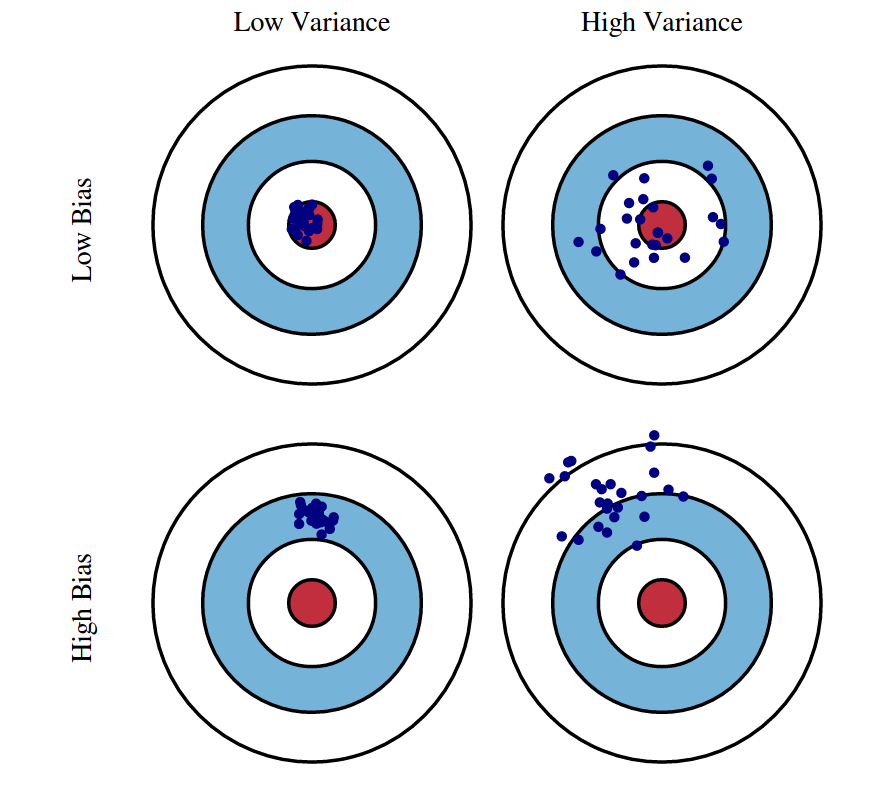
Figure 1: Image from MachineLearningPlus.com
We care about these things because we usually only have our one dataset (when we’re not creating simulated data, that is), but need to know something about how bias and variance tend to look when we change our model complexity.
Deriving Bias and Variance
For this section, recall our model:
\[ y = f(x) + \epsilon \]
This tells us that some of \(y\) can be predicted by the true \(f(x)\), and some is just noise \(\epsilon\). In our simulation from last week, \(f(x) = x^2\), so \(y = x^2 + \epsilon\).
We want to predict \(y\). We call our prediction \(\hat{y}\).
Our best guess for \(f(x)\) is \(\hat{f}(x)\), where \(\hat{f}(x)\) is our model. It might be from a linear regression with 1, 2, 9, 15, etc. predictors or interactions of predictors. It might be from a k-nearest-neighbors estimation with
k = 4. It might be from a regression tree withcp = .1andminsplit=2.Even when we really nail \(\hat{f}(x)\) (which means \(\hat{f}(x) = f(x)\)), there is still error in our prediction because of \(\epsilon\)
- \(y \neq \hat{y}\)
So we think of two different measures of error:
\[ EPE = E[(y - \hat{y})^2] = \underbrace{\mathbb{E}_{\mathcal{D}} \left[ \left(f(x) - \hat{f}(x) \right)^2 \right]}_\textrm{reducible error - MSE from imperfect model} + \underbrace{\mathbb{V}_{Y \mid X} \left[ Y \mid X = x \right]}_{\textrm{irreducible error from }\epsilon} \]
And:
\[ MSE(f(x), \hat{f}(x)) = \mathbb{E}_{\mathcal{D}}\left[\left(f(x) - \hat{f}(x)\right)^2\right] \]
Some of you asked about this equation from last time that decomposed our MSE:
\[ \text{MSE}\left(f(x), \hat{f}(x)\right) = \mathbb{E}_{\mathcal{D}} \left[ \left(f(x) - \hat{f}(x) \right)^2 \right] = \underbrace{\left(f(x) - \mathbb{E} \left[ \hat{f}(x) \right] \right)^2}_{\text{bias}^2 \left(\hat{f}(x) \right)} + \underbrace{\mathbb{E} \left[ \left( \hat{f}(x) - \mathbb{E} \left[ \hat{f}(x) \right] \right)^2 \right]}_{\text{var} \left(\hat{f}(x) \right)} \] This can be derived by:
\[ \begin{eqnarray*} \mathbb{E}_{\mathcal{D}} \left[ \left(f(x) - \hat{f}(x) \right)^2 \right] &=& \mathbb{E}_{\mathcal{D}} \left[\left(f(x) - E[\hat{f}(x)] + E[\hat{f}(x)] - \hat{f}(x)\right)^2 \right] \\ &=& \mathbb{E}_{\mathcal{D}} \left[\left(f(x) - E[\hat{f}(x)]\right)^2 + \left(E[\hat{f}(x)] - \hat{f}(x)\right)^2 + 2\left(f(x) - E[\hat{f}(x)]\right) \left(E[\hat{f}(x)] - \hat{f}(x)\right) \right] \\ &=& \mathbb{E}_{\mathcal{D}} \left[\left(f(x) - E[\hat{f}(x)]\right)^2\right] + \mathbb{E}_{\mathcal{D}} \left[\left(E[\hat{f}(x)] - \hat{f}(x)\right)^2\right] + \mathbb{E}_{\mathcal{D}} \left[2\left(f(x) - E[\hat{f}(x)]\right) \left(E[\hat{f}(x)] - \hat{f}(x)\right) \right] \\ &=& \left(f(x) - E[\hat{f}(x)]\right)^2 + Var\left(\hat{f}(x)\right) + 0 \end{eqnarray*} \] Let’s talk about what’s in this equation:
- MSE is the Mean Squared Error between \(f(x)\) and \(\hat{f}(x)\)
- It does not have the \(\epsilon\) in it
- It is an expectation over all the possible \(\mathcal{D}\) draws of the data we could have
- Because of this \(f(x)\) and \(E\left[\hat{f}(x)\right]\) can move out of the expectation. This lets us cancel that last term with the “2” in it.
The main takeaway is that, even given the error, \(\epsilon\), we still have additional error coming from our inability to perfectly get \(\hat{f}(x) = f(x)\).
A quick bit of R code to help with todays example
We saw before the usefulness of having a list
myList = list()
myList[['thisThing']] = c(1,2,3)
myList[['thisOtherThing']] = c('A','B','C','D')
myList
## $thisThing
## [1] 1 2 3
##
## $thisOtherThing
## [1] "A" "B" "C" "D"It worked really well for holding results from models since we could name the things in the list. But if we put it into a loop:
for(i in c('G','H','I')){
  myList = list()
  myList[[i]] = paste0('This loop is on ',i)
}

print(myList)
## $I
## [1] "This loop is on I"What happened? Every time we used the loop, it re-initiated the list, so we only get the last result!
So what we want is to create the list if it doesn’t exist, and add to it afterwards. We can do that with exists('myList')
for(i in c('G','H','I')){
if(!exists('myList')) myList = list()
myList[[i]] = paste0('This loop is on ',i)
}
print(myList)## $I
## [1] "This loop is on I"
##
## $G
## [1] "This loop is on G"
##
## $H
## [1] "This loop is on H"We’re almost there. It turns out, we have our original \(I\) in there left over from the previous creation of the list. That’s why its out of order. What we want to do is start with a fresh, clean list. If we run rm(myList), the old list will no longer exist, and our code will create a fresh one when we run it again!
rm(myList)
for(i in c('G','H','I')){
if(!exists('myList')) myList = list()
myList[[i]] = paste0('This loop is on ',i)
}
print(myList)## $G
## [1] "This loop is on G"
##
## $H
## [1] "This loop is on H"
##
## $I
## [1] "This loop is on I"You’re going to use this in your groups / breakout rooms today. You’re going to be asked to run some code that stores a plot in a list. To reset the list that stores things, just use rm(listName) (where listName is the name of the list).
Alternatively, you can make sure you run code (outside of the loop) that makes a new list. This will re-set the list to be empty going into the loop:
myList = list()
for(i in c('G','H','I')){
  if(!exists('myList')) myList = list()
  myList[[i]] = paste0('This loop is on ',i)
}
print(myList)
## $G
## [1] "This loop is on G"
##
## $H
## [1] "This loop is on H"
##
## $I
## [1] "This loop is on I"Today’s Example
Our goal today is to
See the code that produced this week’s Content
- Why? Because it helps to illustrate the true sources of noise in the data
See what larger sample sizes and higher/lower irreducible error does to our Bias vs. Variance tradeoff.
Simulation
We will use the exact code from Content 10, which I have reproduced here. I have removed the in-between parts with notation so we can focus on the example. I have copied all of the relevant code into one chunk down at the bottom as well
We’ll need the following libraries:
library(ggplot2)
library(patchwork)
library(tidyverse)
And here, I’ve made a little change to Content 10’s code so we can play with sample size NN and the SD of the irreducible Bayes error.
NN = 100   #----> In class, we will change this to
#                 see how our results change in response
SD.of.Bayes.Error = .75   #-----> This, too, will change.

# Note that both of these are used in the next chunk(s) to generate data.
Begin Content 10 code here:
We will illustrate these decompositions, most importantly the bias-variance tradeoff, through simulation. Suppose we would like to train a model to learn the true regression function function \(f(x) = x^2\).
f = function(x) {
  x ^ 2
}
To carry out a concrete simulation example, we need to fully specify the data generating process. We do so with the following R code.
get_sim_data = function(f, sample_size = NN) {
  x = runif(n = sample_size, min = 0, max = 1)
  eps = rnorm(n = sample_size, mean = 0, sd = SD.of.Bayes.Error)
  y = f(x) + eps
  tibble(x, y)
}
To completely specify the data generating process, we have made more model assumptions than simply \(\mathbb{E}[Y \mid X = x] = x^2\) and \(\mathbb{V}[Y \mid X = x] = \sigma ^ 2\). In particular,
- The \(x_i\) in \(\mathcal{D}\) are sampled from a uniform distribution over \([0, 1]\).
- The \(x_i\) and \(\epsilon\) are independent.
- The \(y_i\) in \(\mathcal{D}\) are sampled from the conditional normal distribution.
Using this setup, we will generate datasets, \(\mathcal{D}\), with a sample size \(NN\) and fit four models.
\[ \begin{aligned} \texttt{predict(fit0, x)} &= \hat{f}_0(x) = \hat{\beta}_0\\ \texttt{predict(fit1, x)} &= \hat{f}_1(x) = \hat{\beta}_0 + \hat{\beta}_1 x \\ \texttt{predict(fit2, x)} &= \hat{f}_2(x) = \hat{\beta}_0 + \hat{\beta}_1 x + \hat{\beta}_2 x^2 \\ \texttt{predict(fit9, x)} &= \hat{f}_9(x) = \hat{\beta}_0 + \hat{\beta}_1 x + \hat{\beta}_2 x^2 + \ldots + \hat{\beta}_9 x^9 \end{aligned} \]
To get a sense of the data and these four models, we generate one simulated dataset, and fit the four models.
set.seed(1)
sim_data = get_sim_data(f)
fit_0 = lm(y ~ 1, data = sim_data)
fit_1 = lm(y ~ poly(x, degree = 1), data = sim_data)
fit_2 = lm(y ~ poly(x, degree = 2), data = sim_data)
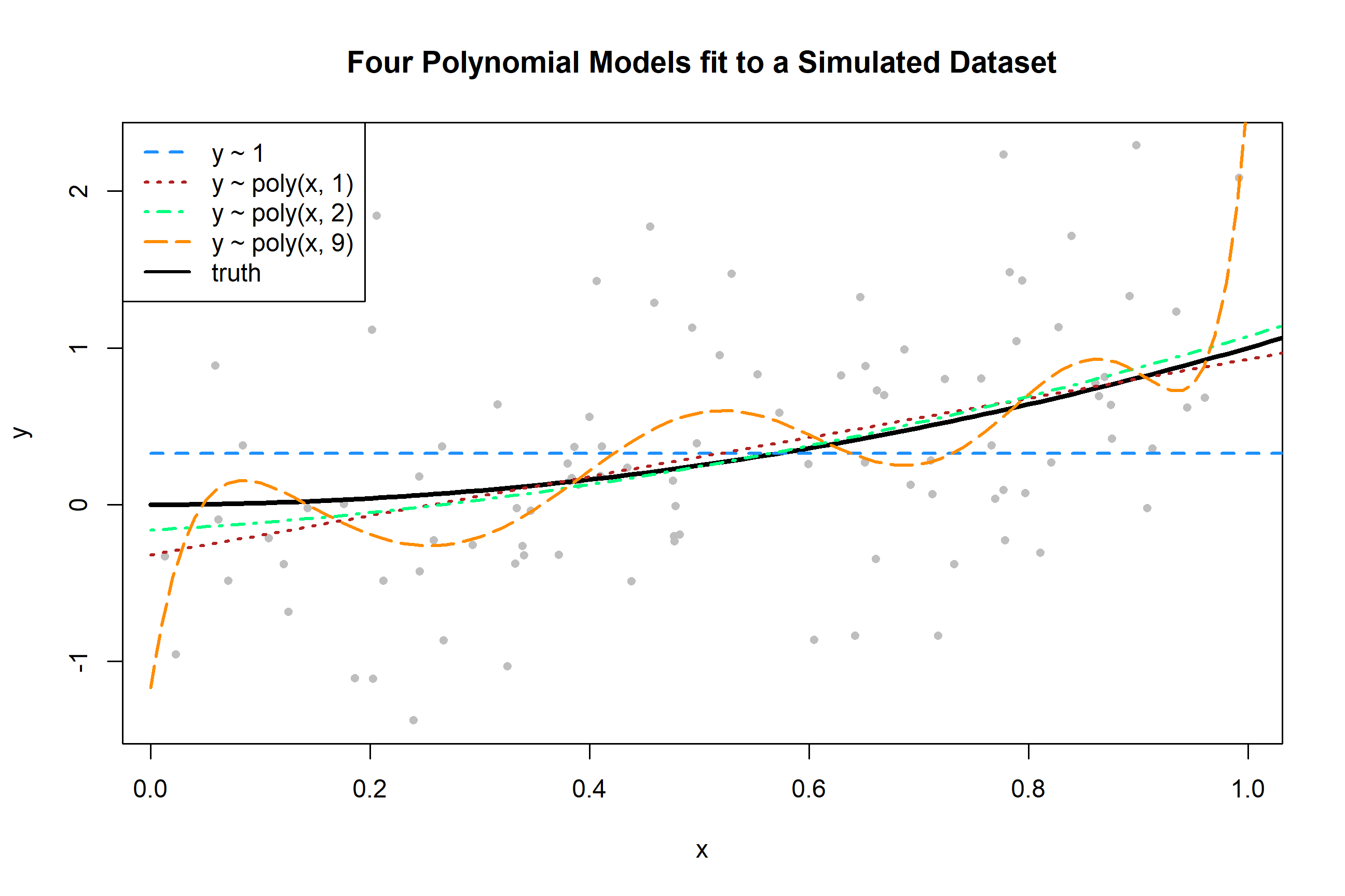
fit_9 = lm(y ~ poly(x, degree = 9), data = sim_data)Plotting these four trained models, we see that the zero predictor model does very poorly. The first degree model is reasonable, but we can see that the second degree model fits much better. The ninth degree model seem rather wild.
…
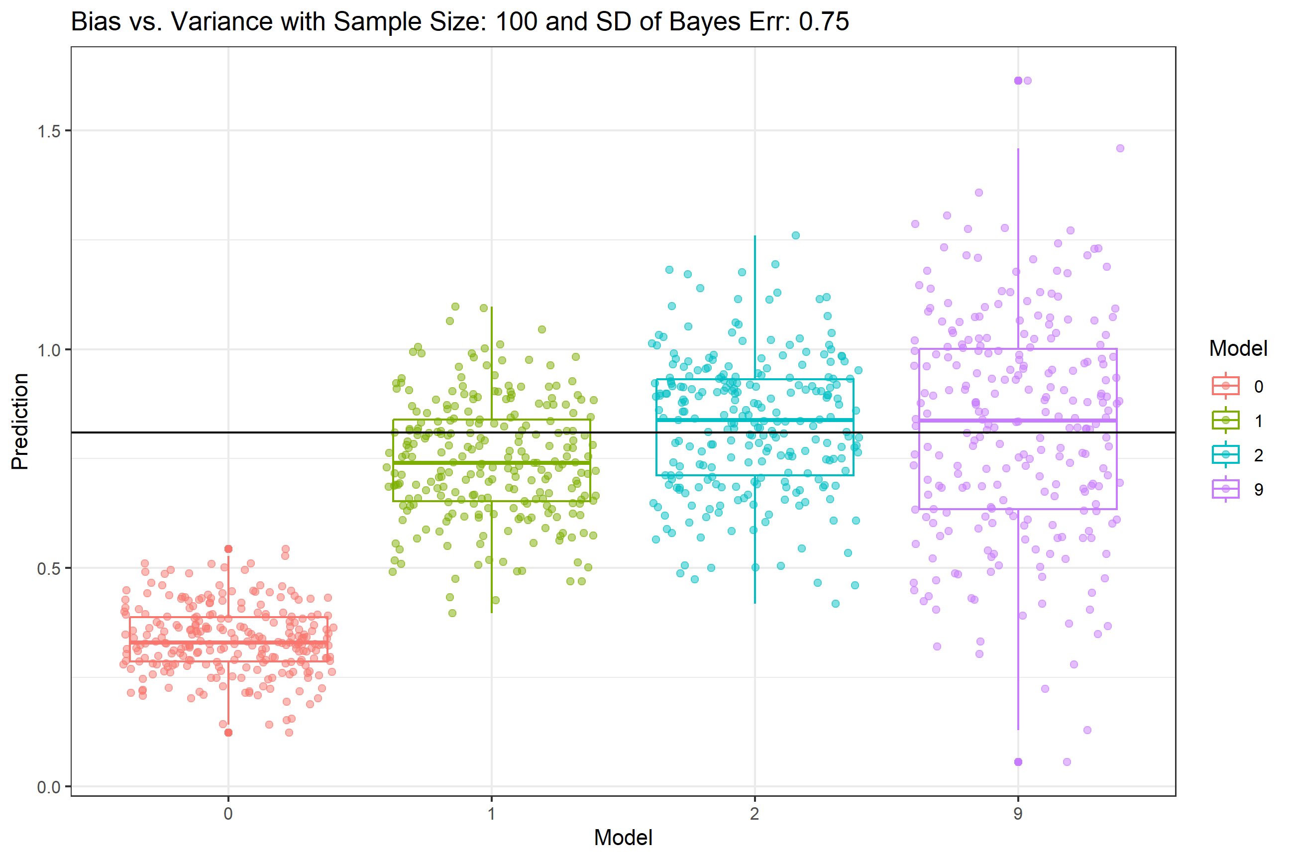
We will now complete a simulation study to understand the relationship between the bias, variance, and mean squared error for the estimates for \(f(x)\) given by these four models at the point \(x = 0.90\). We use simulation to complete this task, as performing the analytical calculations would prove to be rather tedious and difficult.
set.seed(1)
n_sims = 250
n_models = 4
x = data.frame(x = 0.90) # fixed point at which we make predictions
predictions = matrix(0, nrow = n_sims, ncol = n_models)for (sim in 1:n_sims) {
# simulate new, random, training data
# this is the only random portion of the bias, var, and mse calculations
# this allows us to calculate the expectation over D
sim_data = get_sim_data(f, sample_size = NN)
# fit models
fit_0 = lm(y ~ 1,                   data = sim_data)
fit_1 = lm(y ~ poly(x, degree = 1), data = sim_data)
fit_2 = lm(y ~ poly(x, degree = 2), data = sim_data)
fit_9 = lm(y ~ poly(x, degree = 9), data = sim_data)
# get predictions
predictions[sim, 1] = predict(fit_0, x)
predictions[sim, 2] = predict(fit_1, x)
predictions[sim, 3] = predict(fit_2, x)
predictions[sim, 4] = predict(fit_9, x)
}Compile all of the results:
In your group / breakout room and using the code below:
First Breakout: set NN = 100, the value we used in our Content 10 lecture. The value is set in one of the first code chunks. Step through the code to get your finalPlot and make sure it looks like the plot in Content 10. I changed the code to use ggplot (easier to save output), so the formatting and colors will be different - that’s OK, we want to get the same results, not copy the layout of the plot. Note that at the end of the code, a list is created that will hold all of your results. In case you need to clear this list, rm(FinalResults) will do so and the code will initate a new blank list to hold subsequent results.
Second Breakout: set NN to a larger number. Usually, more data means more precise predictions. Run your code again stepping through it, until you get to this plot. Note that at the end of the code provided, there is a list that aggregates your results. Repeat this with a 3rd, even larger value for NN. Don’t go much beyond 50,000 or it’ll take too long. Your FinalResults list should have 3 elements in it. Use patchwork::wrap_plots(FinalResults, nrow = 1) to see all 3 side-by-side.
Third Breakout: Finally, change the SD.of.Bayes.Error value to make it higher or lower. Remember, this is the irreducible error. Run your code again with your first, second, and third different value for sample size NN. You should have 6 plots in your FinalResults list - 3 from before, and 3 more with the new SD of Bayes Error. Use wrap_plots with the right number of rows to see a 2x3 grid of the results.
- Usually we think larger sample sizes and lower error lead to better overall prediction. Do we see any change in the bias vs. tradeoff relationship with lower/higher sample size
NNand lower/higher SD of Bayes Error?
Here’s the code
I’ve merged all of the code together for you here. Copy this into a new .R script - you don’t need to use a full Markdown.
library(ggplot2)
library(patchwork)
library(tidyverse)
NN = 100 #----> In class, we will change this to
# see how our results change in response
SD.of.Bayes.Error = 0.75 #-----> This, too, will change.
# Note that both of these are used in the next chunk(s) to generate data.
f = function(x) {
x ^ 2
}
get_sim_data = function(f, sample_size = NN) {
x = runif(n = sample_size, min = 0, max = 1)
eps = rnorm(n = sample_size, mean = 0, sd = SD.of.Bayes.Error)
y = f(x) + eps
tibble(x, y)
}
## See the fit of the four models (viz only)
set.seed(1)
sim_data = get_sim_data(f)
fit_0 = lm(y ~ 1, data = sim_data)
fit_1 = lm(y ~ poly(x, degree = 1), data = sim_data)
fit_2 = lm(y ~ poly(x, degree = 2), data = sim_data)
fit_9 = lm(y ~ poly(x, degree = 9), data = sim_data)
plot(y ~ x, data = sim_data, col = "grey", pch = 20,
main = "Four Polynomial Models fit to a Simulated Dataset")
grid = seq(from = 0, to = 2, by = 0.01)
lines(grid, f(grid), col = "black", lwd = 3)
lines(grid, predict(fit_0, newdata = data.frame(x = grid)), col = "dodgerblue", lwd = 2, lty = 2)
lines(grid, predict(fit_1, newdata = data.frame(x = grid)), col = "firebrick", lwd = 2, lty = 3)
lines(grid, predict(fit_2, newdata = data.frame(x = grid)), col = "springgreen", lwd = 2, lty = 4)
lines(grid, predict(fit_9, newdata = data.frame(x = grid)), col = "darkorange", lwd = 2, lty = 5)
legend("topleft",
c("y ~ 1", "y ~ poly(x, 1)", "y ~ poly(x, 2)", "y ~ poly(x, 9)", "truth"),
col = c("dodgerblue", "firebrick", "springgreen", "darkorange", "black"), lty = c(2, 3, 4, 5, 1), lwd = 2)
set.seed(1)
n_sims = 250
n_models = 4
x = data.frame(x = 0.90) # fixed point at which we make predictions
predictions = matrix(0, nrow = n_sims, ncol = n_models)
for (sim in 1:n_sims) {

  # simulate new, random, training data
  # this is the only random portion of the bias, var, and mse calculations
  # this allows us to calculate the expectation over D
  sim_data = get_sim_data(f, sample_size = NN)

  # fit models
  fit_0 = lm(y ~ 1,                   data = sim_data)
  fit_1 = lm(y ~ poly(x, degree = 1), data = sim_data)
  fit_2 = lm(y ~ poly(x, degree = 2), data = sim_data)
  fit_9 = lm(y ~ poly(x, degree = 9), data = sim_data)

  # get predictions
  predictions[sim, 1] = predict(fit_0, x)
  predictions[sim, 2] = predict(fit_1, x)
  predictions[sim, 3] = predict(fit_2, x)
  predictions[sim, 4] = predict(fit_9, x)
}
predictions.proc = (predictions)
colnames(predictions.proc) = c("0", "1", "2", "9")
predictions.proc = as.data.frame(predictions.proc)
tall_predictions = tidyr::gather(predictions.proc, factor_key = TRUE)
## Here, you can save your ggplot output
FinalPlot <- ggplot(tall_predictions, aes(x = key, y = value, col = as.factor(key))) +
geom_boxplot() +
geom_jitter(alpha = .5) +
geom_hline(yintercept = f(x = .90)) +
labs(col = 'Model', x = 'Model', y = 'Prediction', title = paste0('Bias v Var - Sample Size: ',NN), subtitle = paste0('SD of Bayes Err: ',SD.of.Bayes.Error)) +
theme_bw()
FinalPlot
## This is going to aggregate your results for you:
if(!exists('FinalResults')) FinalResults = list()
FinalResults[[paste0('finalPlot.NN.',NN,'.SDBayes.',SD.of.Bayes.Error)]] = FinalPlot
# Old plot code:
# boxplot(value ~ key, data = tall_predictions, border = "darkgrey", xlab = "Polynomial Degree", ylab = "Predictions",
# main = "Simulated Predictions for Polynomial Models")
# grid()
# stripchart(value ~ key, data = tall_predictions, add = TRUE, vertical = TRUE, method = "jitter", jitter = 0.15, pch = 1, col = c("dodgerblue", "firebrick", "springgreen", "darkorange"))
# abline(h = f(x = 0.90), lwd = 2)And to output whatever is in your list of ggplot objects:
## This not run automatically.
## To plot the whole list of ggplot objects in FinalResults:
patchwork::wrap_plots(FinalResults, nrow = 2, guides = 'collect')