Nonparametric Regression
Our data and goal
We want to use the wooldridge::wage2 data on wages to generate and tune a non-parametric model of wages using a regression tree (or decision tree, same thing). Use ?wage2 (after you’ve loaded the wooldridge package) to see the data dictionary.
We’ve learned that our RMSE calculations have a hard time with NAs in the data. So let’s use the skim output to tell us which variables have too many NA (see n_missing) values and should be dropped. Let’s set a high bar here, and drop anything that isn’t 100% complete. Of course, there are other things we can do (impute the NAs, or make dummies for them), but for now, it’s easiest to drop them.
Remember, skim() is for your own exploration, it’s not something that you should include in your output.
Once cleaned, we should be able to use rpart(wage ~ ., data = wage_clean) and not have any NAs in our prediction. That’s what we’ll do in our first Breakout.
Breakout #1 - Predicting Wage
I’m going to have you form groups of 2-3 to work on live-coding. One person in the group will need to have Rstudio up, be able to share screen, and have the correct packages loaded (caret, rpart, and rpart.plot, plus skimr). Copy the rmse and get_rmse code into a blank R script (you don’t have to use RMarkdown, just use a blank R script and run from there). You’ll also want to have these functions from last week loaded:
rmse = function(actual, predicted) {
  sqrt(mean((actual - predicted) ^ 2))
}
get_rmse = function(model, data, response) {
rmse(actual = subset(data, select = response, drop = TRUE),
predicted = predict(model, data))
}For the first breakout, all I want you to do is the following. We are trying to predict wage for this exercise:
- Estimate a default regression tree on
wage_cleanusing the default parameters (use the whole dataset for now, we’ll train-test on the problem set). - Use
rpart.plotto vizualize your regression tree, and talk through the interpretation with each other. - Calculate the RMSE for your regression tree.
We’ll spend about 5 minutes on this. Remember, you can use ?wage2 to see the variable names. Make sure you know what variables are showing up in the plot and explaining wage in your model. You may find something odd at first and may need to drop more variables…
5 minutes
Breakout #1 discussion
Let’s choose a group to share their plot and discuss the results. Use our sharing zoom link: bit.ly/KIRKPATRICK
Automating models
Let’s talk about a little code shortcut that helps iterate through your model selection.
First, before, we used list() to store all of our models. This is because list() can “hold” anything at all, unlike a matrix, which is only numeric, or a data.frame which needs all rows in a column to be the same data type. list() is also recursive, so each element in a list can be a list. Of lists. Of lists!
Lists are also really easy to add to iteratively. We can initiate an empty list using myList <- list(), then we can add things to it. Note that we use the double [ to index:
myList <- list()
myList[['first']] = 'This is the first thing on my list'
print(myList)
## $first
## [1] "This is the first thing on my list"Lists let you name the “containers” (much like you can name colums in a data.frame). Our first one is called “first”. We can add more later, but they always have to be unique:
myList[['second']] = c(1,2,3)
print(myList)
## $first
## [1] "This is the first thing on my list"
##
## $second
## [1] 1 2 3And still more:
myList[['third']] = data.frame(a = c(1,2,3), b = c('Albert','Alex','Alice'))
print(myList)
## $first
## [1] "This is the first thing on my list"
##
## $second
## [1] 1 2 3
##
## $third
## a b
## 1 1 Albert
## 2 2 Alex
## 3 3 AliceNow we have a data.frame in there! We can use lapply to do something to every element in the list:
lapply(myList, length) # the length() function with the first entry being the list element## $first
## [1] 1
##
## $second
## [1] 3
##
## $third
## [1] 2We get back a list of equal length but each (still-named) container is now the length of the original list’s contents.
Loops
R has a very useful looping function that takes the form:
for(i in c('first','second','third')){
print(i)
}
## [1] "first"
## [1] "second"
## [1] "third"Here, R is repeating the thing in the loop (print(i)) with a different value for i each time. R repeats only what is inside the curly-brackets, then when it reaches the close-curly-bracket, it goes back to the top, changes i to the next element, and repeats.
We can use this to train our models. First, we clear our list object myList by setting it equal to an empty list. Then, we loop over some regression tree tuning parameters. First, we have to figure out how to use the loop to set a unique name for each list container. To do this, we’ll use paste0('Tuning',i) which will result in a character string of Tuning0 when i=0, Tuning0.01 when i=0.01, etc.
myList <- list()   # resets the list. Otherwise, you'll just be adding to your old list!

for(i in c(0, 0.01, 0.02)){
  myList[[paste0('Tuning',i)]] = rpart(wage ~ ., data = wage_clean, cp = i)
}
If you use names(myList) you’ll see the result of our paste0 naming. If you want to see the plotted results, you can use:
rpart.plot(myList[['Tuning0.01']])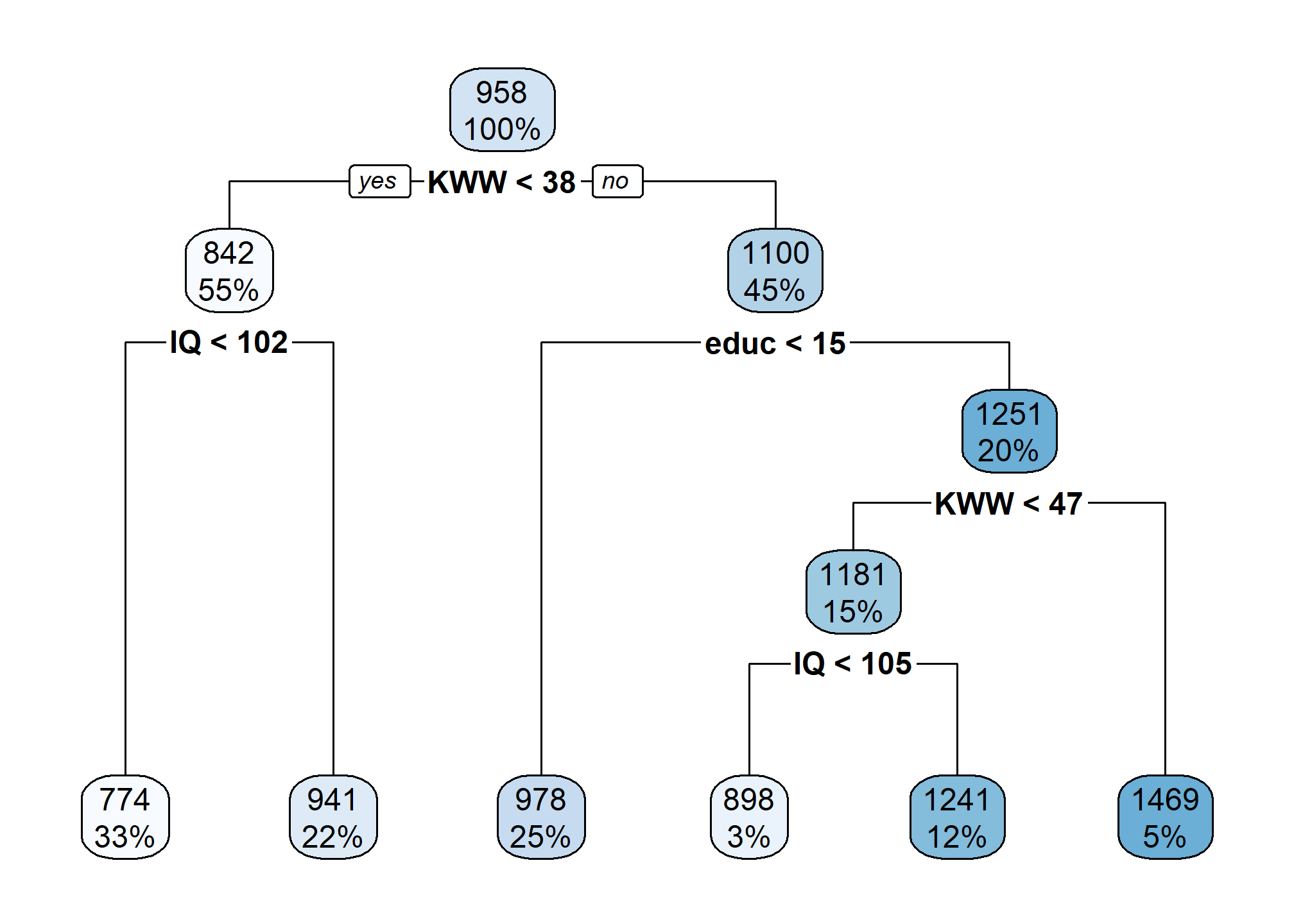
Using lapply to repeat something
Once we have a list built, lapply lets us do something to each element of the list, and then returns a list of results (of the same length as the input).
Note that in the above myList, we don’t actually have the cp parameter recorded anywhere except in the name of the list element. If we want to plot with cp on the x-axis, we’d need to have the number. Later on, we’ll cover text as data and learn how to extract it, but an easier way is to lapply a function that extracts the cp used over the list.
You can retrieve the cp and minsplit arguments from the tree by noting that the rpart object is itself technically a list, and it has an element called control that is itself a list, and that list has cp and minsplit as used in the estimation. You can use the $ accessor on lists:
myTree = myList[[2]]

myTree$control$cp
## [1] 0.01The only problem here is that we don’t have a function written that does $control$cp. We can use an anonymous function in lapply as follows:
cp_list = lapply(myList, function(x){
  x$control$cp
})

unlist(cp_list)
## Tuning0 Tuning0.01 Tuning0.02
## 0.00 0.01 0.02Well, it gets us the right answer, but whaaaaaat is going on? Curly brackets? x?
This is an “anonymous function”, or a function created on the fly. Here’s how it works in lapply:
- The first argument is the list you want to do something to
- The second argument would usually be the function you want to apply, like
get_rmse - Here, we’re going to ask R to temporarily create a function that takes one argument,
x. xis going to be each list element inmyList.- Think of it as a loop:
- Take the first element of
myListand refer to it asx. Run the function’s code. - Then it’ll take the second element of
myListand refer to it asxand run the function’s code. - Repeat until all elements of
xhave been used.
- Take the first element of
- Once the anonymous function has been applied to
x, the result is passed back and saved as the new element of the list output, always in the same position from where thexwas taken.
So you can think of it like this:
x = myList[[1]]
myList[[1]] = x$control$cp

x = myList[[2]]
myList[[2]] = x$control$cp

x = myList[[3]]
myList[[3]] = x$control$cp
As long as every entry in myList is an rpart object with control$cp, then you’ll get those values in a list. unlist just coerces the list to a vector. This is also the same way we get the RMSE, but instead of the anonymous function, we write one out and use that.
Lab 7
In Lab 7, linear models, you were asked to make increasingly complex models by adding variables. In regression trees and kNN, complexity comes from a tuning parameter. But many people have asked about ways of doing Lab 7, so here are two possible solutions.
Solution 1: Make a list of models
First, we make a vector of all of our possible explanatory variables:
wagenames = names(wage2)
wagenames = wagenames[!wagenames %in% c('wage','lwage')]
wagenames
## [1] "hours" "IQ" "KWW" "educ" "exper" "tenure" "age"
## [8] "married" "black" "south" "urban" "sibs" "brthord" "meduc"
## [15] "feduc"And we’ll do all the interactions, quadratic terms, and put them all in one long vector:
wagenamesintx = expand.grid(wagenames, wagenames)
wagenamesintx = paste0(wagenamesintx[,1], ':', wagenamesintx[,2])

wagenamessquared = paste0(wagenames, '^2')

wageparameters = c(wagenames, wagenamesintx, wagenamessquared)
wageparameters[c(1,10,100,200)] # just to see a few
## [1] "hours" "south" "south:tenure" "exper:brthord"Now we need to make a list of formulas that start with wage ~ and include an ever-increasing number of entries in wageparameters (and, to be nested, always includes the previous iteration). We’ll do this by taking an index of [1:N] where N gets bigger.
There are 255 possible entries, so we want to sequence along that and always need round numbers:
complexity = round(seq(from = 1, to = length(wageparameters),  length.out = 15))

modelList = lapply(complexity, function(x){
  list_formula_start = 'wage ~ '
  list_formula_rhs = paste0(wageparameters[1:x], collapse = ' + ')
  return(paste0(list_formula_start, list_formula_rhs))
})

print(modelList[1:3])
## [[1]]
## [1] "wage ~ hours"
##
## [[2]]
## [1] "wage ~ hours + IQ + KWW + educ + exper + tenure + age + married + black + south + urban + sibs + brthord + meduc + feduc + hours:hours + IQ:hours + KWW:hours + educ:hours"
##
## [[3]]
## [1] "wage ~ hours + IQ + KWW + educ + exper + tenure + age + married + black + south + urban + sibs + brthord + meduc + feduc + hours:hours + IQ:hours + KWW:hours + educ:hours + exper:hours + tenure:hours + age:hours + married:hours + black:hours + south:hours + urban:hours + sibs:hours + brthord:hours + meduc:hours + feduc:hours + hours:IQ + IQ:IQ + KWW:IQ + educ:IQ + exper:IQ + tenure:IQ + age:IQ"Finally, we start using lapply to estimate the model:
myOLS = lapply(modelList, function(y){
  lm(y, data = wage2)
})

lapply(myOLS[1:3], summary)
## [[1]]
##
## Call:
## lm(formula = y, data = wage2)
##
## Residuals:
## Min 1Q Median 3Q Max
## -839.72 -287.21 -52.38 200.46 2131.26
##
## Coefficients:
## Estimate Std. Error t value Pr(>|t|)
## (Intercept) 981.315 81.575 12.03 <2e-16 ***
## hours -0.532 1.832 -0.29 0.772
## ---
## Signif. codes: 0 '***' 0.001 '**' 0.01 '*' 0.05 '.' 0.1 ' ' 1
##
## Residual standard error: 404.6 on 933 degrees of freedom
## Multiple R-squared: 9.033e-05, Adjusted R-squared: -0.0009814
## F-statistic: 0.08429 on 1 and 933 DF, p-value: 0.7716
##
##
## [[2]]
##
## Call:
## lm(formula = y, data = wage2)
##
## Residuals:
## Min 1Q Median 3Q Max
## -823.41 -209.85 -36.73 169.56 1945.67
##
## Coefficients:
## Estimate Std. Error t value Pr(>|t|)
## (Intercept) -333.4545 673.8072 -0.495 0.620853
## hours -12.1500 14.0223 -0.866 0.386553
## IQ 8.4166 6.9960 1.203 0.229395
## KWW -16.7569 12.7468 -1.315 0.189112
## educ 29.6737 48.0285 0.618 0.536903
## exper 9.9812 4.4862 2.225 0.026435 *
## tenure 2.9739 2.9258 1.016 0.309808
## age 8.9932 6.0635 1.483 0.138520
## married 178.8599 46.4966 3.847 0.000132 ***
## black -100.5218 56.4193 -1.782 0.075271 .
## south -23.3841 31.0616 -0.753 0.451828
## urban 179.0588 31.5547 5.675 2.1e-08 ***
## sibs 8.6548 7.9696 1.086 0.277895
## brthord -18.0249 11.7300 -1.537 0.124871
## meduc 7.1703 6.2323 1.151 0.250362
## feduc 8.8008 5.4714 1.609 0.108214
## hours:IQ -0.1226 0.1566 -0.783 0.434026
## hours:KWW 0.4812 0.2801 1.718 0.086282 .
## hours:educ 0.1991 1.0457 0.190 0.849036
## ---
## Signif. codes: 0 '***' 0.001 '**' 0.01 '*' 0.05 '.' 0.1 ' ' 1
##
## Residual standard error: 354.1 on 644 degrees of freedom
## (272 observations deleted due to missingness)
## Multiple R-squared: 0.262, Adjusted R-squared: 0.2414
## F-statistic: 12.7 on 18 and 644 DF, p-value: < 2.2e-16
##
##
## [[3]]
##
## Call:
## lm(formula = y, data = wage2)
##
## Residuals:
## Min 1Q Median 3Q Max
## -876.85 -208.34 -41.58 184.31 1964.55
##
## Coefficients:
## Estimate Std. Error t value Pr(>|t|)
## (Intercept) 2526.42104 1778.98063 1.420 0.15606
## hours -28.84096 27.34871 -1.055 0.29203
## IQ -11.05195 14.41481 -0.767 0.44354
## KWW -32.51353 21.95935 -1.481 0.13921
## educ -65.27306 87.11894 -0.749 0.45399
## exper -56.47871 43.73030 -1.292 0.19700
## tenure 61.99723 27.55945 2.250 0.02482 *
## age -20.60242 53.42036 -0.386 0.69987
## married 174.59592 291.22705 0.600 0.54904
## black 129.07837 389.95580 0.331 0.74075
## south -219.74759 209.99378 -1.046 0.29576
## urban 294.24907 215.20016 1.367 0.17201
## sibs 33.26592 57.47098 0.579 0.56291
## brthord -12.35032 81.74380 -0.151 0.87996
## meduc -14.65740 42.07236 -0.348 0.72767
## feduc 45.44872 37.63676 1.208 0.22767
## hours:IQ -0.13457 0.17547 -0.767 0.44345
## hours:KWW 0.50497 0.31608 1.598 0.11064
## hours:educ 1.70417 1.35782 1.255 0.20992
## hours:exper 1.28802 0.68683 1.875 0.06121 .
## hours:tenure -1.23958 0.44602 -2.779 0.00561 **
## hours:age -0.12173 0.82131 -0.148 0.88222
## hours:married 0.10483 6.63109 0.016 0.98739
## hours:black -5.90930 8.93377 -0.661 0.50856
## hours:south 4.48976 4.76877 0.941 0.34681
## hours:urban -2.64292 4.85060 -0.545 0.58604
## hours:sibs -0.59065 1.30658 -0.452 0.65138
## hours:brthord -0.14475 1.88695 -0.077 0.93888
## hours:meduc 0.54974 0.95729 0.574 0.56600
## hours:feduc -0.86832 0.83946 -1.034 0.30136
## IQ:KWW 0.14886 0.15533 0.958 0.33823
## IQ:educ 0.24425 0.57544 0.424 0.67138
## IQ:exper 0.09552 0.31666 0.302 0.76302
## IQ:tenure -0.04357 0.20709 -0.210 0.83342
## IQ:age 0.32399 0.41337 0.784 0.43347
## ---
## Signif. codes: 0 '***' 0.001 '**' 0.01 '*' 0.05 '.' 0.1 ' ' 1
##
## Residual standard error: 353.2 on 628 degrees of freedom
## (272 observations deleted due to missingness)
## Multiple R-squared: 0.2838, Adjusted R-squared: 0.2451
## F-statistic: 7.32 on 34 and 628 DF, p-value: < 2.2e-16Breakout #2
Using the loop method or the lapply method, generate 10 regression trees to explain wage in wage_clean. You can iterate through values of cp, the complexity parameter, or minsplit, the minimum # of points that have to be in each split.
10 minutes
Breakout #2 discussion
We’ll ask someone to share (a few of) their group’s 10 regression trees using rpart.plot. Use bit.ly/KIRKPATRICK to volunteer to share.
Breakout #3 (if time)
Use lapply to get a list of your RMSE’s (one for each of your models). The anonymous function may come in handy here (though it’s not necessary). Note that we are not yet splitting into test and train (which you will need to do on your lab assignment).
Once you have your list, create the plot of RMSEs similar to the one we looked at in Content this week. Note: you can use unlist(myRMSE) to get a numeric vector of the RMSE’s (as long as all of the elements in myRMSE are numeric). Then, it’s a matter of plotting either with base plot or with ggplot (if you use ggplot you’ll have to tidy the RMSE by adding the index column or naming the x-axis).