Welcome Back to R
Readings
As noted in the syllabus, your readings will be assigned each week in this area. For this initial week, please read the course content. Read closely the following:
Guiding Question
For future lectures, the guiding questions will be more pointed and at a higher level to help steer your thinking. Here, we want to ensure you remember some basics and accordingly the questions are straightforward.
- How does this course work?
- Do you remember anything about
R? - What are the different data types in
R? - How do you index specific elements of a vector? Why might you want to do that?
A Brief Introduction to SSC442
About Me
Me: My primary area of expertise is environmental and energy (applied) economics.
This class is totally, unapologetically a work in progress. It was developed mainly by Prof. Bushong with refinements by myself.
Material is a mish-mash of stuff from courses offered at Caltech, Stanford, Harvard, and Duke…so, yeah, it will be challenging. Hopefully, you’ll find it fun!
My research: occasionally touches the topics in the course, but mostly utilizes things in the course as tools.
About You
New phone who dis? Please email me jkirk@msu.edu with the subject [SSC442] Who Dis. In the message, tell me:
name (with pronunciation guide)
major
desired graduation year and semester
interest in this course on a 10-point scale (1: not at all interested; 10: helllllll yeah)
You must spend 5 minutes emailing me a little bit about your interests before the next class. This counts towards your “participation” grade (more on that later)
This Course
The syllabus is posted on the course website. I’ll walk through highlights now, but read it later – it’s long.
- But eventually, please read it. It is required.
Syllabus highlights:
- Grade is composed of weekly writings, labs, and projects (see syllabus page for exact points)
- Weekly writings: 19%
- Participation: 4%
- Labs: 32%
- Projects: 45%
- This structure is designed to give ~55% “for free”. Success on the projects will require real work.
- Labs consist of a practical implementation of something we’ve covered in the course (e.g., code your own Recommender System).
Course Structure
Here’s how each week will work: before class on Tuesday, you’ll read the content for the week. On Tuesday, you’ll come to lecture. Before Thursday, you’ll read the example for the week, and on Thursday you’ll come to lecture ready to participate with a charged laptop. On Saturday night by 11:59pm, you’ll turn in your Weekly Writing assignment responding to the weekly writing prompt given during class on Tuesday or Thursday, rendered to PDF by RMarkdown and using the proper template (see assignments). By Monday at 11:59pm, you’ll turn in your Lab assignment, also using the RMarkdown template.
You’ll repeat this each week until we’re out of labs. If a holiday occurs on a due date, then the assignment or lab is due the next non-holiday day at 11:59pm. You’ll also work with your assigned group on the Group Project. We’ll assign groups after the drop deadline has passed.
Now, let’s look at the Syllabus for important information about office hours
Grading
Grading: come to class.
If you complete all assignments and attend all class dates, I suspect you will do very well. Given the way the syllabus is structured, I conjecture that the following is a loose guide to grades:
4.0 Turned in all assignments with good effort, worked hard on the projects and was proud of final product.
3.5 Turned in all assignments with good effort, worked a bit on the projects and was indifferent to final product.
3.0 Turned in all assignments with some effort, worked a bit on the projects and was shy about final product.
< 3.0 Very little effort, or did not turn in all assignments, worked very little on the projects and was embarassed by final product.
…of course, failing to turn in assignments can lead to a grade dramatically lower than just a 3.0.
More About This Course
There are sort of two texts for this course and sort of zero.
The “main text” is this website. The secondary text is Introduction to Statistical Learning (see Syllabus), which is free and available online. The secondary text is substantially more difficult, but also free online. Assigned readings can be found on the course website under “Content”.
Please please please please please: ask questions during class.
Most ideas will be new.
Sometimes (often?) the material itself will be confusing or interesting—or both!
Teaching online is incredibly challenging (no feedback) and chat is vital to success.We’re back in person and I/we have a healthy aversion to zoom!Note: If I find that attendance is terrible, I may have to start incorporating attendance into participation.
Return of the Please: If there is some topic that you really want to learn about, ask. If you are uncomfortable asking in front of the whole group, please see me during office hours.
Because this is a new-ish course:
Some of the lectures will be way too long or too short.
Some of the lectures won’t make sense at first
Some of the time I’ll forget what I intended to say and awkwardly stare at you for a few moments (sorry).
Comment throughout the course, not just at the end.
I encourage measured feedback and thoughtful responses to questions. If I call on you and you don’t know immediately, don’t freak out. If you don’t know, it’s totally okay to say you don’t know.
SUPER BIG IMPORTANT EXPLANATION OF THE COURSE
I teach using “math”.
…Don’t be afraid. The math won’t hurt you.
I fundamentally believe that true knowledge of how we learn from data depends on a basic understanding of the underlying mathematics.
-Good news: no black boxes.
You’ll actually learn stuff. (Probably. Hopefully?)
Also good news: level of required math is reasonably low. High-school algebra or equivalent should be fine.
-Bad news: some notation-heavy slides and reading.
And finally…
Finally: I cannot address field-specific questions in areas outside economics to any satisfying degree.
Good news: I’m good at knowing what I don’t know and have a very small ego, which means that I’m much less likely to blow smoke up your rear than other professors.
Bad news: I can’t help with certain types of questions.
This course should be applicable broadly, but many of the examples will lean on my personal expertise (sorry).
Your assignment: read syllabus, the content from Week 0 if you haven’t already, and the Example from Week 0 for Thursday. Make sure R and RStudio is running on your computer or you have a RStudio.cloud/Posit.cloud account, and make sure you can knit your Rmarkdown template to PDF. Do your weekly writing due Saturday. Begin working on Lab 0 as it is due Monday.
Things to stress from syllabus:
- E-mail isn’t the ideal solution for technical problems
- If you do send an email, please start it with
[SSC442]and the subject.
- If you do send an email, please start it with
- No appointments necessary for regularly scheduled office hours; or by appointment and via Slack
- TA office hours are great as well. Our TA has experience in this course.
- Notify me immediately if you need accommodations because of RCPD or religious convictions; If you approach me at the last minute, I may not be able to help.
Despite my hard-assness in these intro slides: I’m here to help and I am not in the business of giving bad grades for no reason.
What is “Data Analytics”?
I keep saying that the sexy job in the next 10 years will be statisticians. And I’m not kidding.
Hal Varian, Chief Economist, Google
How do you define “data analytics”? (Not a rhetorical question!)
- This course will avoid this nomenclature. It is confusing and imprecise. But you signed up (suckers) and I owe an explanation of what this course will cover.
Some “data analytics” topics we will cover:
- Linear regression: il classico.
- LASSO
- Models of classification or discrete choice.
- Analysis of ``wide’’ data.
- Decision trees and other non-linear models.
Starting point for this course
Better utilizing existing data can improve our predictive power whilst providing interpretable outputs for considering new policies.
WARNING: Causation is tough and we will spend the entire course warning you to avoid making causal claims!
The Pros and Cons of Correlation
Pros:
- Nature gives you correlations for free.
- In principle, everyone can agree on the facts.
Cons:
- Correlations are not very helpful.
- They show what has happened, but not why.
- For many things, we care about why. The social science perspective asks “why?”
Why a Correlation Exists Between X and Y
\(X \rightarrow Y\) X causes Y (causality)
\(X \leftarrow Y\) Y causes X (reverse causality)
\(Z \rightarrow X\); \(Z \rightarrow Y\) Z causes X and Y (common cause)
\(X \rightarrow Y\); \(Y \rightarrow X\) X causes Y and Y causes X (simultaneous equations)
A Case Study in Prediction
Example: a firm wishes to predict user behavior based on previous purchases or interactions.
Small margins \(\rightarrow\) huge payoffs when scaled up.
\(.01\% \rightarrow\) $10 million.
Not obvious why this was true for Netflix; quite obvious why this is true in financial markets.
From a computer science perspective, it only matters that you get that improvement ($$). From a social science perspective, we would want to use the predictions to learn more about why.
More Recent Examples of Prediction
- Identify the risk factors for prostate cancer.
- Classify a tissue sample into one of several cancer classes, based on a gene expression profile.
- Classify a recorded phoneme based on a log-periodogram.
- Predict whether someone will have a heart attack on the basis of demographic, diet and clinical measurements.
- Customize an email spam detection system.
- Identify a hand-drawn object.
- Determine which oscillations of stellar luminosity are likely due to exoplanets.
- Identify food combinations that cause spikes in blood glucose level for an individual.
- Establish the relationship between salary and demographic variables in population survey data.
An Aside: Nomenclature
Machine learning arose as a subfield of Artificial Intelligence.
Statistical learning arose as a subfield of Statistics.
There is much overlap; however, a few points of distinction:
Machine learning has a greater emphasis on large scale applications and prediction accuracy.
Statistical learning emphasizes models and their interpretability, and precision and uncertainty.
- But the distinction has become more and more blurred, and there is a great deal of “cross-fertilization”.
Obviously true: machine learning has the upper hand in marketing.
Learning from Data
The following are the basic requirements for statistical learning:
- A pattern exists.
- This pattern is not easily expressed in a closed mathematical form.
- You have data.
Case study: US homicides by firearm
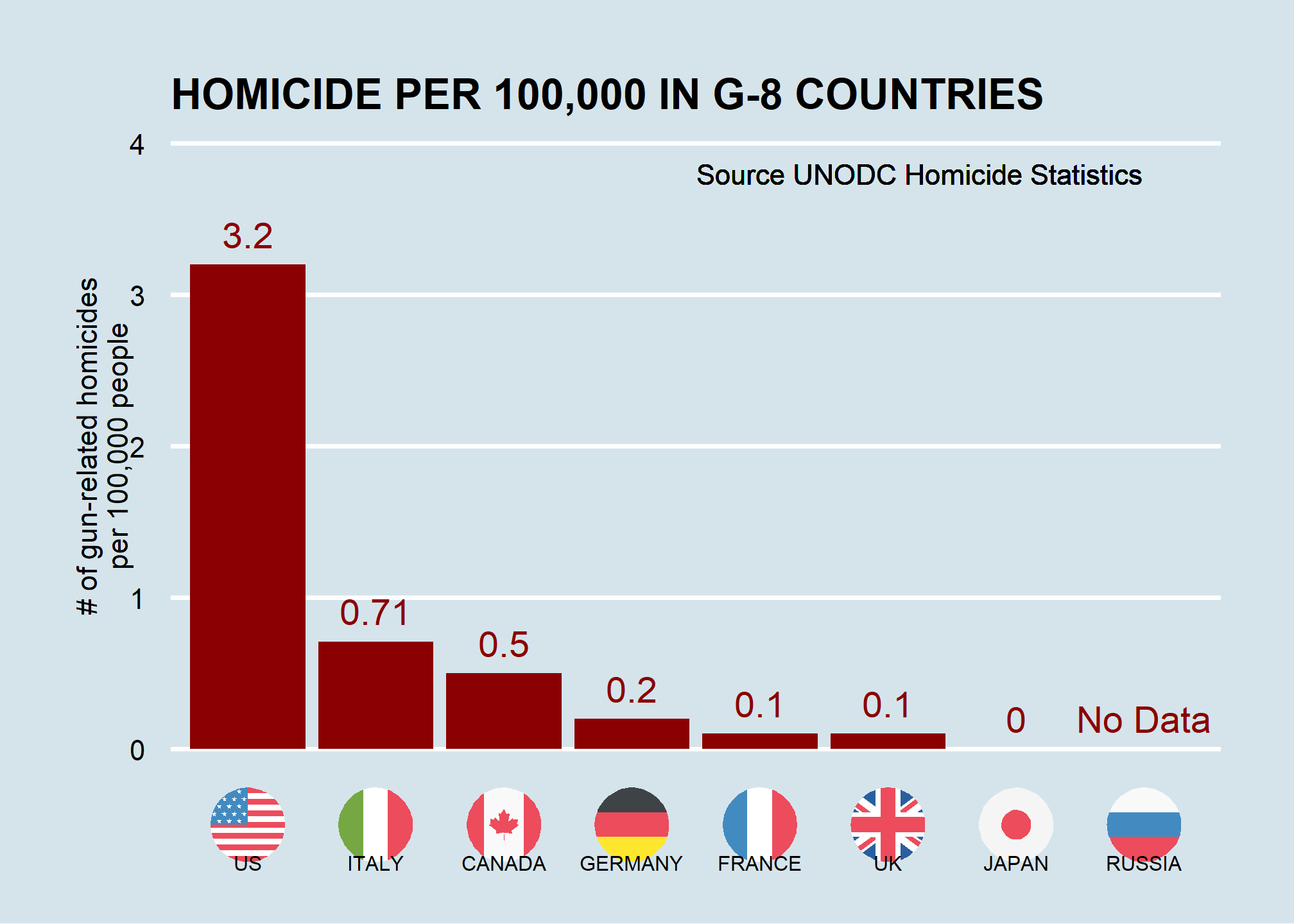
Imagine you live in Europe (if only!) and are offered a job in a US company with many locations in every state. It is a great job, but headlines such as US Gun Homicide Rate Higher Than Other Developed Countries1 have you worried. Fox News runs a scary looking graphic, and charts like the one below only add to that concern:
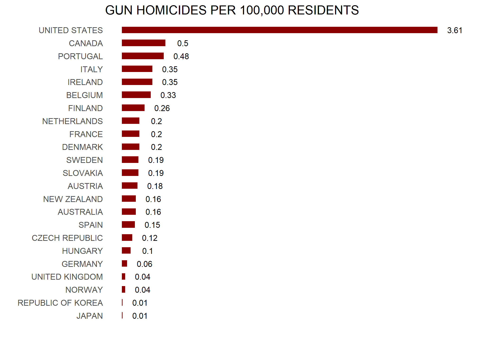
Or even worse, this version from everytown.org:
But then you remember that (1) this is a hypothetical exercise; (2) you’ll take literally any job at this point; and (3) Geographic diversity matters – the United States is a large and diverse country with 50 very different states (plus the District of Columbia and some lovely territories).2
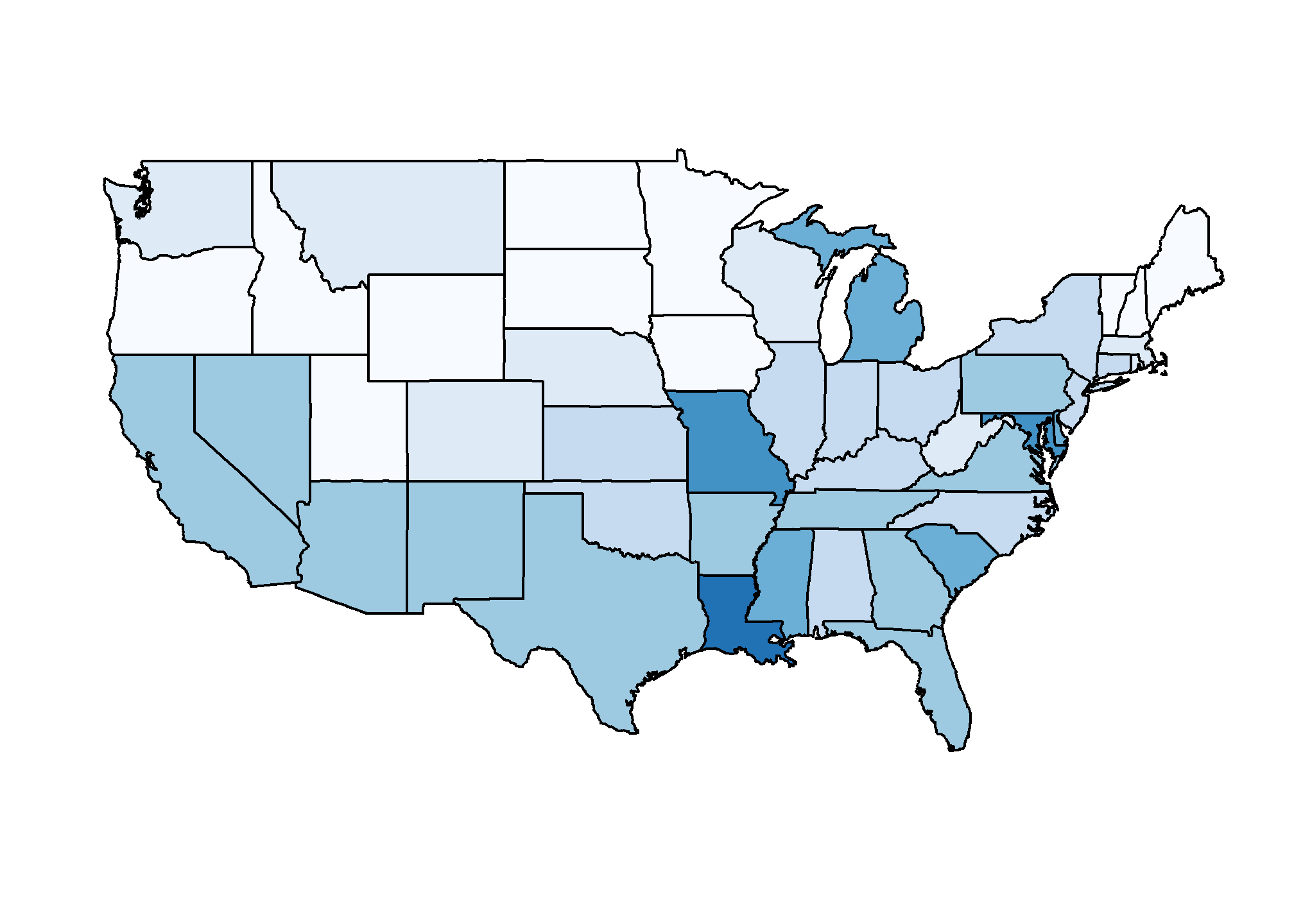
California, for example, has a larger population than Canada, and 20 US states have populations larger than that of Norway. In some respects, the variability across states in the US is akin to the variability across countries in Europe. Furthermore, although not included in the charts above, the murder rates in Lithuania, Ukraine, and Russia are higher than 4 per 100,000. So perhaps the news reports that worried you are too superficial.
This is a relatively simple and straightforward problem in social science: you have options of where to live, and want to determine the safety of the various states. Your “research” is clearly policy-relevant: you will eventually have to live somewhere. In this course, we will begin to tackle the problem by examining data related to gun homicides in the US during 2010 using R as a motivating example along the way.
Before we get started with our example, we need to cover logistics as well as some of the very basic building blocks that are required to gain more advanced R skills. Ideally, this is a refresher. However, we are aware that your preparation in previously courses varies greatly from student to student. Moreover, we want you to be aware that the usefulness of some of these early building blocks may not be immediately obvious. Later in the class you will appreciate having these skills. Mastery will be rewarded both in this class and (of course) in life.
Let’s pause here for questions
Getting started with R and RStudio Posit Workflows
In Content this week, we reviewed the use of R. Now, let’s talk about doing work in R.
R is not a programming language like C or Java. It was not created by software engineers for software development. Instead, it was developed by statisticians as an interactive environment for data analysis. You can read the full history in the paper A Brief History of S3. The interactivity is an indispensable feature in data science because, as you will soon learn, the ability to quickly explore data is a necessity for success in this field. However, like in other programming languages, you can save your work as scripts that can be easily executed at any moment. These scripts serve as a record of the analysis you performed, a key feature that facilitates reproducible work. If you are an expert programmer, you should not expect R to follow the conventions you are used—assuming this will leave you disappointed. If you are patient, you will come to appreciate the unequal power of R when it comes to data analysis and data visualization.
Other attractive features of R are:
Ris free and open source4.- It runs on all major platforms: Windows, Mac OS, UNIX/Linux.
- Scripts and data objects can be shared seamlessly across platforms.
- There is a large, growing, and active community of
Rusers and, as a result, there are numerous resources for learning and asking questions5 6 7. - It is easy for others to contribute add-ons which enables developers to share software implementations of new data science methodologies. The latest methods and tools are developed in
Rfor a wide variety of disciplines and since social science is so broad,Ris one of the few tools that spans the varied social sciences.
Installing R and RStudio Posit
If you have not yet done so, you’ll need to install both R and RStudio/Posit (as we mentioned before, RStudio is undergoing a change in name). See the Installing page of our course resources for instructions.
I have created a video walkthrough for the basics of using R for another course, but it is useful here. You can see part A here (labeled “Part 2a”) here ] and part B here (labeled “Part 2b”) . You should already be at this level of familiarity with R, but if you need a review, this is a good place to start.
The R console
Interactive data analysis usually occurs on the R console that executes commands as you type them. There are several ways to gain access to an R console. One way is to simply start R on your computer. R Studio runs R inside of, so you won’t usually access R this way. The console looks something like this:
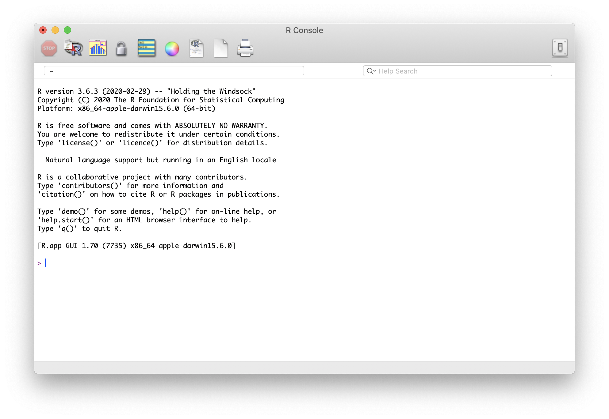
As a quick example, try using the console to calculate a 15% tip on a meal that cost $19.71:8
0.15 * 19.71 ## [1] 2.9565Note that in this course (at least, on most browsers), grey boxes are used to show R code typed into the R console. The symbol ## is used to denote what the R console outputs.
Scripts
One of the great advantages of R over point-and-click analysis software is that you can save your work as scripts. You can edit and save these scripts using a text editor. The material in this course was developed using the interactive integrated development environment (IDE) RStudio9. RStudio includes an editor with many R specific features, a console to execute your code, and other useful panes, including one to show figures.
Most web-based R consoles also provide a pane to edit scripts, but not all permit you to save the scripts for later use. On the upper-right part of this webpage you’ll see a little button with the R logo. You can access a web-based console there.
RStudio
RStudio (undergoing a re-brand to “Posit”) will be our launching pad for data science projects. It not only provides an editor for us to create and edit our scripts but also provides many other useful tools. In this section, we go over some of the basics.
The panes
When you start RStudio for the first time, you will see three panes. The left pane shows the R console. On the right, the top pane includes tabs such as Environment and History, while the bottom pane shows five tabs: File, Plots, Packages, Help, and Viewer (these tabs may change in new versions). You can click on each tab to move across the different features.
To start a new script, you can click on File, then New File, then R Script.
This starts a new pane on the left and it is here where you can start writing your script.
Key bindings
Many tasks we perform with the mouse can be achieved with a combination of key strokes instead. These keyboard versions for performing tasks are referred to as key bindings. For example, we just showed how to use the mouse to start a new script, but you can also use a key binding: Ctrl+Shift+N on Windows and command+shift+N on the Mac.
Although in this tutorial we often show how to use the mouse, we highly recommend that you memorize key bindings for the operations you use most. RStudio provides a useful cheat sheet with the most widely used commands. You might want to keep this handy so you can look up key-bindings when you find yourself performing repetitive point-and-clicking.
Running commands while editing scripts
There are many editors specifically made for coding. These are useful because color and indentation are automatically added to make code more readable. RStudio is one of these editors, and it was specifically developed for R. One of the main advantages provided by RStudio over other editors is that we can test our code easily as we edit our scripts. Below we show an example.
Let’s start by opening a new script as we did before. A next step is to give the script a name. We can do this through the editor by saving the current new unnamed script. To do this, click on the save icon or use the key binding Ctrl+S on Windows and command+S on the Mac.
When you ask for the document to be saved for the first time, RStudio will prompt you for a name. A good convention is to use a descriptive name, with lower case letters, no spaces, only hyphens to separate words, and then followed by the suffix .R. We will call this script my-first-script.R.
Now we are ready to start editing our first script. The first lines of code in an R script are dedicated to loading the libraries we will use. Another useful RStudio feature is that once we type library() it starts auto-completing with libraries that we have installed. Note what happens when we type library(ti):
Another feature you may have noticed is that when you type library( the second parenthesis is automatically added. This will help you avoid one of the most common errors in coding: forgetting to close a parenthesis.
Now we can continue to write code. As an example, we will make a graph showing murder totals versus population totals by state. Once you are done writing the code needed to make this plot, you can try it out by executing the code. To do this, click on the Run button on the upper right side of the editing pane. You can also use the key binding: Ctrl+Shift+Enter on Windows or command+shift+return on the Mac.
Once you run the code, you will see it appear in the R console and, in this case, the generated plot appears in the plots console. Note that the plot console has a useful interface that permits you to click back and forward across different plots, zoom in to the plot, or save the plots as files.
To run one line at a time instead of the entire script, you can use Control-Enter on Windows and command-return on the Mac.
SETUP TIP
Change the option Save workspace to .RData on exit to Never and uncheck the Restore .RData into workspace at start. By default, when you exit R saves all the objects you have created into a file called .RData. This is done so that when you restart the session in the same folder, it will load these objects. I find that this causes confusion especially when sharing code with colleagues or peers.
Installing R packages
The functionality provided by a fresh install of R is only a small fraction of what is possible. In fact, we refer to what you get after your first install as base R. The extra functionality comes from add-ons available from developers. There are currently hundreds of these available from CRAN and many others shared via other repositories such as GitHub. However, because not everybody needs all available functionality, R instead makes different components available via packages. R makes it very easy to install packages from within R. For example, to install the dslabs package, which we use to share datasets and code related to this course, you would type directly into the console:
install.packages("dslabs")In RStudio, you can navigate to the Tools tab and select install packages. We can then load the package into our R sessions using the library function:
library(dslabs)As you go through this course, you will see that we load packages without installing them. This is because once you install a package, it remains installed and only needs to be loaded with library. The package remains loaded until we quit the R session. If you try to load a package and get an error, it probably means you need to install it first.
This also means that strange things can happen if you add install.packages() to a script – you’ll be re-installing the package every time you run the script, and that will lead to errors. Lots of them. So you install the packages once and only once on your computer via the packages pane or directly in the console, then you never install that package again.
We can install more than one package at once by feeding a character vector to this function:
install.packages(c("tidyverse", "dslabs"))One advantage of using RStudio is that it auto-completes package names once you start typing, which is helpful when you do not remember the exact spelling of the package. Once you select your package, we recommend selecting all the defaults. Note that installing tidyverse actually installs several packages. This commonly occurs when a package has dependencies, or uses functions from other packages. When you load a package using library, you also load its dependencies.
Once packages are installed, you can load them into R and you do not need to install them again, unless you install a fresh version of R. Remember packages are installed in R not RStudio.
It is helpful to keep a list of all the packages you need for your work in a script because if you need to perform a fresh install of R, you can re-install all your packages by simply running a script.
You can see all the packages you have installed using the following function:
installed.packages()As we move through this course, we will constantly be adding to our toolbox of packages. Accordingly, you will need to keep track to ensure you have the requisite package for any given lecture.
Rmarkdown
Markdown is a general-purpose syntax for laying out documents. Rmarkdown is a combination of R and markdown, as the name implies. When using markdown, one can define headers and tables using specific notation, and depending on the rendering engine, the headers and tables (and a whole lot more) are customized. In fact, this whole website is built in R using Rmarkdown (and a lot of add-ons like Hugo and blogdown). In other contexts, the rendering engine may recognize that your headers are likely to be entries in a table of contents, and does so for you. The table of contents at the top of this document is built from the markdown headers.
The power of Rmarkdown is that it lets us mix formatted text with R code. That is, you can have a section of the document that understands R code, and a separate section right after that discusses the results from the R code.
Try it out using the Weekly Writing Template from the Assignments tab. If it opens in your web browser, just right-click the link and select Save As…. Make sure you save the file to its own folder on your hard drive. In converting your Rmarkdown .Rmd file to a .pdf, your system will make multiple interim files10. It also creates folders to store the output of any plots or graphics you create with your R code.
If you’re new to Rmarkdown, I have made a short video on how to use it . This video is for my EC420 course, but works for us as well.
To use Rmarkdown, you’ll have to install a few packages (like knitr and tinytex) and you’ll have to install a copy of LaTeX installed. Follow these instructions if you haven’t ever used RMarkdown with LaTeX to install LaTeX.
If we have time today, let’s open the template linked above and see what happens when we select “knit to pdf”. If you do not wind up with a PDF rendered using LaTeX that looks like the one below, then check for errors. The most common one is not having tinytex and latex installed (tinytex will install a light version of latex).
Screentshot of header of PDF file properly rendered
http://abcnews.go.com/blogs/headlines/2012/12/us-gun-ownership-homicide-rate-higher-than-other-developed-countries/↩︎
I’m especially partial to Puerto Rico.↩︎
https://pdfs.semanticscholar.org/9b48/46f192aa37ca122cfabb1ed1b59866d8bfda.pdf↩︎
https://stats.stackexchange.com/questions/138/free-resources-for-learning-r↩︎
But probably tip more than 15%. Times are tough, man.↩︎
Specifically, knitr will create an intermediate .md file which is then processed with Pandoc using Latex to create a pdf. Whew!↩︎
Social Science Approaches to Statistical Learning
A Brief History
Suppose you are a researcher and you want to know whether prisons reduce crime.
from “A Call for a Moratorium on Prison Building” (1976)